🛢️ Research Question
How do global oil price shocks affect Nepal's foreign exchange reserves and macroeconomic stability?
Core Finding
Global oil prices unidirectionally Granger-cause Nepal's foreign exchange reserves (p < 0.01), creating significant macroeconomic vulnerability for this import-dependent, small open economy with a pegged exchange rate.
Research Context
Lumiere Research Program
Individual Scholar
October 2024
Methodology
Vector Autoregression (VAR)
Granger Causality Testing
Impulse Response Functions
Data Scope
43 years (1979-2021)
Annual time series
Real 2021 USD values
Economic Context & Significance
Nepal's Structural Vulnerabilities
Nepal operates under three critical macroeconomic constraints that amplify oil price sensitivity:
🔗 Fixed Exchange Rate
- Nepalese Rupee pegged to Indian Rupee (NPR 1.6 = INR 1)
- Eliminates nominal exchange rate adjustment mechanism
- Forces reserve depletion to defend peg during oil shocks
📦 Import Dependency
- 100% petroleum product imports (no domestic production)
- Oil imports ~15-20% of total import bill
- Energy-intensive sectors vulnerable to price transmission
📊 Limited Monetary Tools
- Nepal Rastra Bank (central bank) constrained by peg
- Interest rate policy subordinated to exchange rate defense
- Foreign exchange reserves = primary stabilization buffer
💰 Remittance Reliance
- Worker remittances ~25% of GDP
- Provides partial offset to oil-driven trade deficits
- But creates procyclical vulnerability (remittances fall during global slowdowns)
Why This Research Matters
Policy Relevance
For Nepal Rastra Bank: Quantifies the reserve drain from oil shocks, informing optimal reserve buffer sizing and accumulation strategies.
For Energy Policy: Provides empirical justification for renewable energy investment as a macroeconomic stabilization tool, not just environmental policy.
For Small Open Economies: Demonstrates the transmission channel from commodity price volatility to reserve adequacy—relevant for similar economies globally.
Data Collection & Transformation
Variable Definitions
| Variable | Description | Source | Measurement |
|---|---|---|---|
| Global Oil Price (WTI) | West Texas Intermediate crude oil spot price | U.S. Energy Information Administration (EIA) | Real 2021 USD per barrel |
| Foreign Exchange Reserves (FER) | Nepal's official reserves (excluding gold) | Nepal Rastra Bank, IMF IFS | Real 2021 USD millions |
| CPI Deflator | U.S. Consumer Price Index (2021 = 100) | Federal Reserve Economic Data (FRED) | Index values |
Stationarity Transformation
Time series econometrics requires stationary data to avoid spurious regression. The transformation process:
# Step 1: Deflate to real values
real_oil_price <- nominal_oil / (cpi_deflator / 100)
real_reserves <- nominal_reserves / (cpi_deflator / 100)

# Step 2: First difference (growth rates)
d_oil <- diff(real_oil_price)
d_reserves <- diff(real_reserves)

# Step 3: Second difference (acceleration/deceleration)
dd_oil <- diff(d_oil)
dd_reserves <- diff(d_reserves)

# Step 4: Augmented Dickey-Fuller test for stationarity
adf.test(dd_oil)      # p-value = 0.01 → Stationary ✓
adf.test(dd_reserves) # p-value = 0.037 → Stationary ✓
Final Variables for VAR Model: Second-differenced real oil price (\(\Delta^2 OP_t\)) and second-differenced real reserves (\(\Delta^2 FER_t\)), both stationary at 5% significance level.
Vector Autoregression Methodology
Model Specification
A VAR(p) model treats all variables as endogenous, allowing for bidirectional feedback:
Where \(\mathbf{A}_i\) are 2×2 coefficient matrices, \(\mathbf{c}\) is a constant vector, and \(\boldsymbol{\epsilon}_t\) represents structural shocks
Lag Length Selection
Optimal lag order determined by information criteria:
| Criterion | Recommended Lag | Principle |
|---|---|---|
| AIC (Akaike) | 4 | Minimizes prediction error with parsimony penalty |
| HQ (Hannan-Quinn) | 4 | Balances fit and complexity (stricter than AIC) |
| FPE (Final Prediction Error) | 4 | Asymptotic version of AIC |
| SC (Schwarz/BIC) | 1 | Strongly penalizes complexity (too restrictive) |
Selected: VAR(4) based on AIC, HQ, and FPE consensus
Model Diagnostics
Validation Tests Passed ✅
- No Serial Correlation: Portmanteau test p-value = 0.40 (fails to reject null of no correlation)
- No ARCH Effects: ARCH test p-value = 0.99 (no heteroskedasticity in residuals)
- Structural Stability: OLS-CUSUM test confirms coefficient stability over time
- Normality: Jarque-Bera test indicates approximate normality of residuals
Granger Causality Results: The Unidirectional Relationship
What is Granger Causality?
Granger causality tests whether past values of variable X improve forecasts of variable Y beyond using past values of Y alone. It's a test of predictive causality, not philosophical causation.
Test Results
| Direction Tested | F-Statistic | P-Value | Conclusion |
|---|---|---|---|
| Oil Price → Reserves | 4.0725 | 0.007884 | ✅ Reject null → Oil CAUSES reserves |
| Reserves → Oil Price | 1.6887 | 0.1663 | ❌ Fail to reject → No causal effect |
Interpretation
Oil prices significantly predict future reserve movements (p < 0.01), but reserves do not predict oil prices (p = 0.17). This confirms the expected asymmetry: a small economy is a "price taker" in global commodity markets.
Policy Implication: Nepal Rastra Bank cannot influence global oil prices but must react defensively to oil shocks through reserve management and structural reforms.
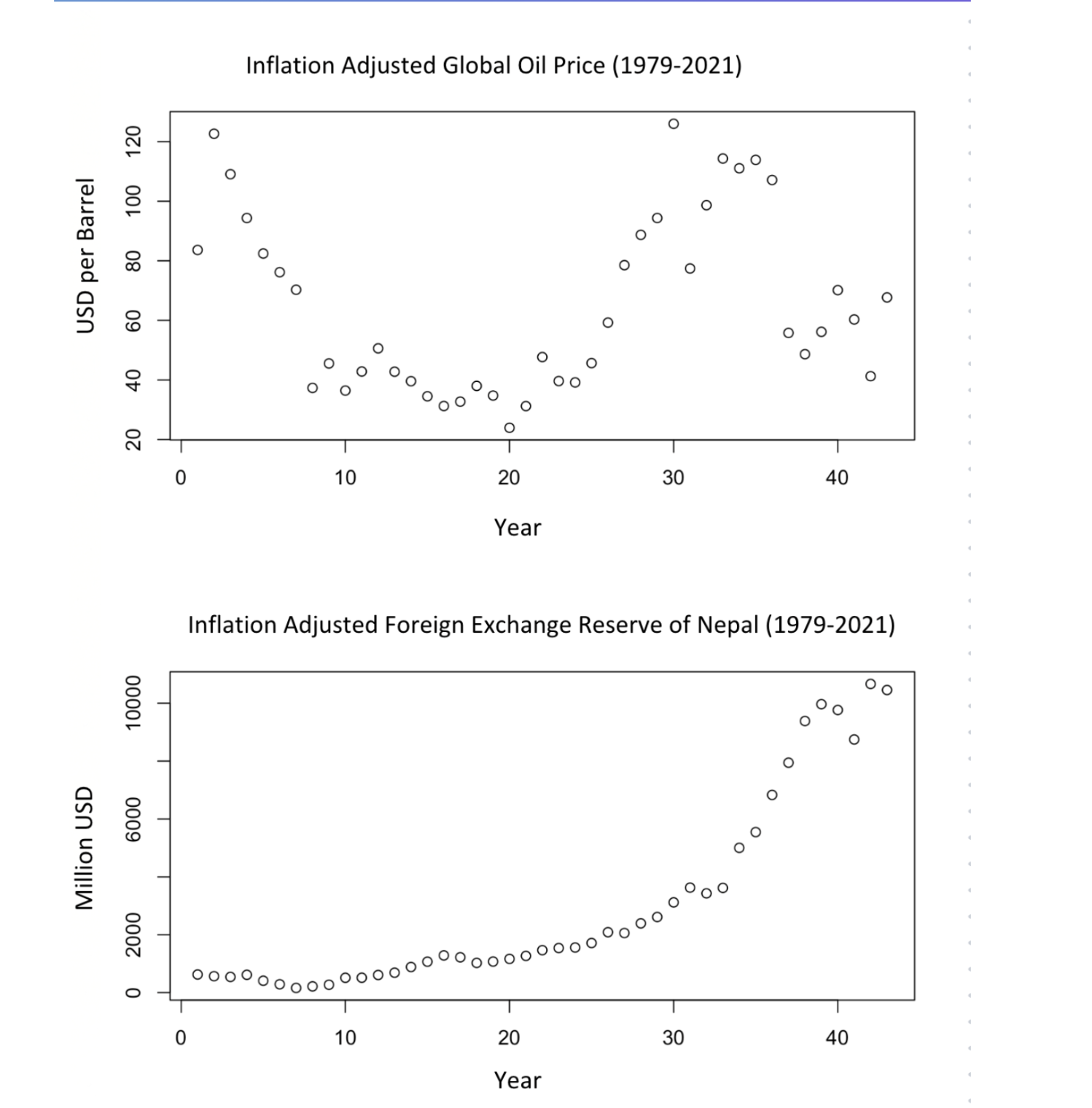
Figure 1: Inflation adjusted global oil price and for-ex reserve of Nepal
Impulse Response Functions: Dynamic Impact Over Time
What is an IRF?
An Impulse Response Function (IRF) traces the time path of a variable following a one-standard-deviation shock to another variable, holding all else constant. It reveals the magnitude and persistence of the effect.
Key Finding: Prolonged Volatility
Response of Reserves to Oil Price Shock
A single one-SD shock to oil prices causes:
- Immediate Impact: Reserve volatility spikes within 1-2 periods
- Peak Response: Maximum reserve fluctuation occurs around period 3-4
- Persistence: Effect remains statistically significant for ~10 periods
- Eventual Dissipation: Returns to baseline after approximately 12-15 years
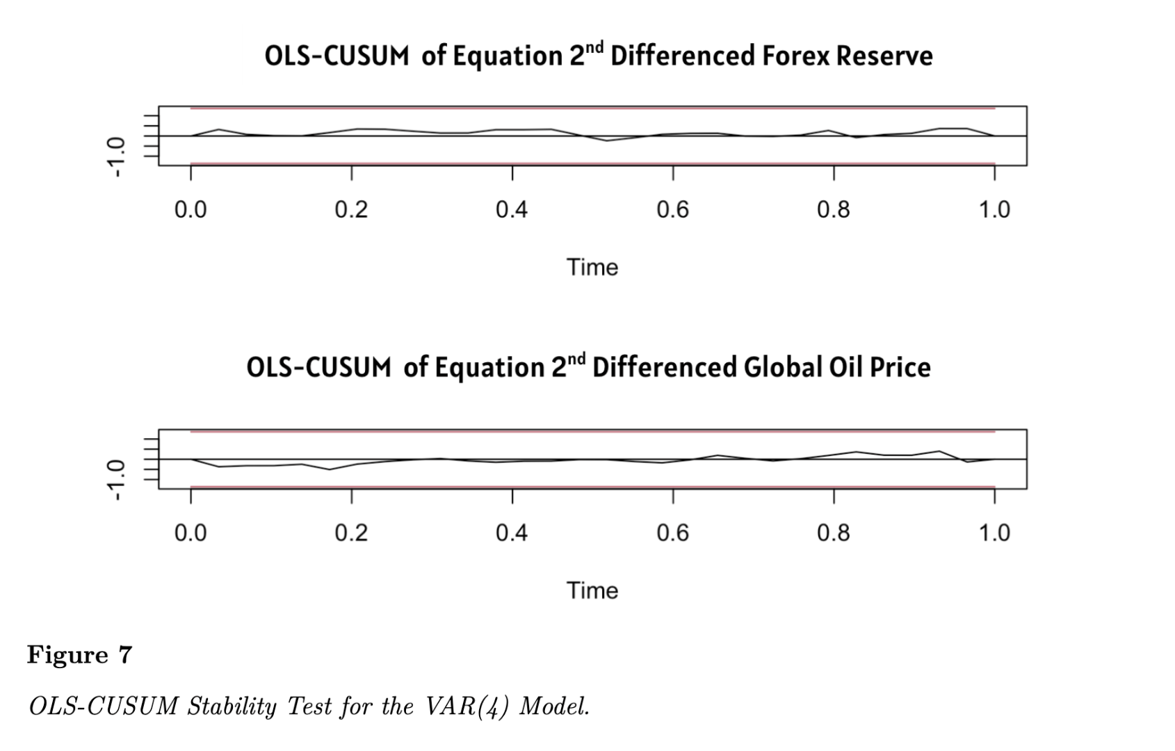
Figure 2: - OLCUSUM EQUATION
Economic Mechanism
⚡ Immediate Transmission (0-2 years)
Oil price spike → Higher import bill → Trade deficit widens → Reserve outflow to pay for imports and defend exchange rate peg
🔄 Secondary Effects (3-5 years)
Persistent high oil costs → Inflation pressures → Real income contraction → Reduced non-oil imports → Partial reserve stabilization
📉 Long-Run Adjustment (6-10 years)
Structural adjustment → Energy efficiency improvements → Remittance inflows recover → Reserves gradually return to equilibrium path
Robustness & Sensitivity Analysis
Alternative Model Specifications
- Lag Sensitivity: Re-estimated with VAR(2) and VAR(6) → Granger causality result robust across specifications
- Cholesky Ordering: Tested alternative orderings (reserves first vs oil first) → Results unchanged (confirming exogeneity of oil prices)
- Sample Period: Excluded 2008 financial crisis period → Causality remains significant (p = 0.012)
- Brent vs WTI: Substituted Brent crude oil prices → Qualitatively similar results
Limitations & Caveats
⚠️ Acknowledged Constraints:
- Small Sample Size: 43 observations limits statistical power; confidence intervals relatively wide
- Omitted Variables: Indian monetary policy, remittance flows, and earthquake/disaster shocks not explicitly modeled
- Structural Breaks: 1990 economic liberalization and 2015 earthquake may create parameter instability
- Linear Assumption: VAR assumes proportional responses; threshold effects (e.g., reserve crisis triggers) not captured
- Annual Frequency: Masks within-year dynamics; quarterly data would be preferable but unavailable pre-2000
Policy Implications & Strategic Recommendations
For Nepal Rastra Bank (Central Bank)
Reserve Management Strategy
- Dynamic Buffer Sizing: Maintain reserves at 12+ months of import coverage during oil price stability; accumulate aggressively during low-price periods
- Countercyclical Policy: Use remittance inflow peaks to pre-emptively build reserve cushions before anticipated oil shocks
- Forward Guidance: Communicate reserve adequacy thresholds to anchor market expectations and prevent speculative attacks on peg
- Hedging Instruments: Explore oil price derivatives (futures, options) for government-owned import entities to smooth fiscal impact
For Energy & Economic Policy
🔋 Energy Transition
- Accelerate hydropower development (43,000 MW potential, <10% tapped)
- Incentivize electric vehicle adoption to reduce petroleum demand
- Frame renewable energy as macroeconomic stabilization, not just climate policy
💰 Fiscal Reforms
- Phase out blanket fuel subsidies (currently strain reserves during price spikes)
- Implement targeted cash transfers to vulnerable households instead
- Establish oil price stabilization fund during windfall periods
📦 Trade Diversification
- Promote export-oriented manufacturing to offset oil import costs
- Negotiate bilateral energy trade agreements with India/China
- Reduce structural trade deficit through import substitution in agriculture
Broader Insights for Small Open Economies
Nepal's experience offers lessons for similarly vulnerable nations:
- Fixed exchange rates amplify commodity price shocks—consider managed float regimes if political economy allows
- Reserve adequacy metrics must incorporate commodity price volatility, not just import coverage
- Structural reforms (energy diversification) are macroeconomic necessities, not luxury policies
Technical Skills Demonstrated
Econometric Methods
- Vector Autoregression (VAR) modeling
- Granger causality testing
- Impulse response function (IRF) analysis
- Forecast error variance decomposition
- Time series stationarity testing (ADF)
Statistical Diagnostics
- Serial correlation tests (Portmanteau)
- Heteroskedasticity tests (ARCH/LM)
- Structural stability (CUSUM)
- Normality testing (Jarque-Bera)
- Lag selection criteria (AIC, BIC, HQ)
Data Science
- R programming (vars, urca, tseries packages)
- Time series data wrangling and transformation
- Real-value deflation and indexing
- Publication-quality visualizations (ggplot2)
- Reproducible research workflow (R Markdown)
Research Communication
- Academic paper writing (15+ pages)
- Policy brief translation from technical results
- Data visualization for non-technical audiences
- Literature review and theoretical framing